You draw your CFA model, click Calculate Estimates and get CFI = 0.86 and RMSEA = 0.091, or worse, AMOS says “The model is probably unidentified”. Adding a few covariance arrows makes the numbers look better, but is that legitimate? This AMOS tutorial for your thesis follows the full process, from CFA to model fit, validity, SEM, mediation and multi-group analysis, with the ways of improving fit that stand up to scrutiny and how to fix AMOS’s common errors.
- What AMOS is and how it differs from SPSS and SmartPLS
- Preparing your data in SPSS
- CFA: confirmatory factor analysis
- Model fit: which indices, which thresholds?
- Poor model fit: how to improve it legitimately
- Convergent and discriminant validity
- The structural model (SEM)
- Testing mediation with bootstrap
- Multi-group analysis
- Common AMOS errors and fixes
1What AMOS is and how it differs from SPSS and SmartPLS
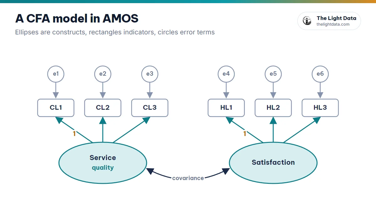
AMOS (Analysis of Moment Structures) is IBM’s structural equation modeling software, which comes with IBM SPSS Statistics. You build and test a model by drawing it: latent variables are ellipses, observed variables are rectangles and relationships are arrows.
Compared with SPSS
SPSS is strong in traditional statistics (alpha, EFA, regression); AMOS tests many relationships at once, accounts for measurement error, and gives direct, indirect and total effects.
Compared with SmartPLS
AMOS uses CB-SEM, suited to confirming theory with a full set of fit indices; it needs larger samples and near-normal data. See the full comparison →
2Preparing your data in SPSS before AMOS
AMOS reads .sav files directly. Before you start:
- Clean the data: handle missing values, outliers and invalid responses. Bootstrap and modification indices require complete data.
- Run Cronbach’s alpha and remove items with an item-total correlation below 0.3.
- Run EFA to check the factor structure (Principal Axis Factoring with Promax is often recommended before CFA).
- Save the .sav file with short variable names.
3CFA: confirmatory factor analysis
CFA tests your measurement model: whether observed items really measure the latent variables your theory says they do. Unlike EFA, which explores, CFA is used when you already have a clear theoretical structure. It gives you model fit, convergent and discriminant validity, CR and AVE.
- Open AMOS Graphics → File → Data Files → link your .sav file.
- Draw each latent variable with its indicators using Draw a latent variable or add an indicator. AMOS adds the error terms and fixes one loading to 1.
- Name indicators to match your .sav variables (drag them from List variables in data set).
- Add covariances (two-headed arrows) between the latent variables.
- Analysis Properties → Output: tick Standardized estimates, Squared multiple correlations and Modification indices.
- Analyze → Calculate Estimates → View Text Output.
4Model fit in AMOS: which indices, which thresholds?
| Index | Common threshold | Stricter (Hu & Bentler, 1999) |
|---|---|---|
| CMIN/DF | < 3 (or < 5) | — |
| CFI | ≥ 0.90 | ≥ 0.95 |
| TLI | ≥ 0.90 | ≥ 0.95 |
| RMSEA | ≤ 0.08 | ≤ 0.06 |
| SRMR | ≤ 0.08 | ≤ 0.08 |
| GFI | ≥ 0.90 (≥ 0.80 accepted by some authors) | — |
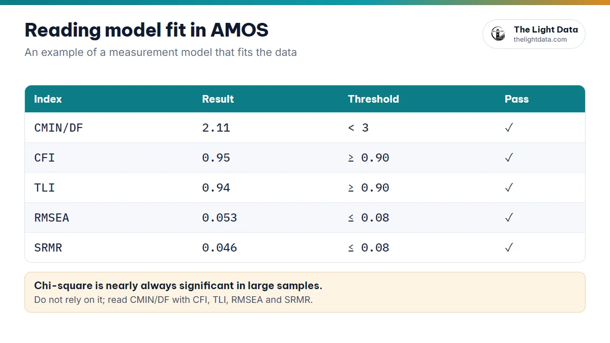
- Chi-square is nearly always significant in large samples, so do not rely on it. Read CMIN/DF together with CFI, TLI, RMSEA and SRMR.
- GFI and AGFI are sensitive to sample size; many authors now prefer CFI, TLI, RMSEA and SRMR.
- SRMR is not in the Text Output by default: use Plugins → Standardized RMR, then run the model again.
CMIN/DF = 2.11, CFI = 0.95, TLI = 0.94, RMSEA = 0.053, SRMR = 0.046: the measurement model fits the data.
5Poor model fit: how to improve it legitimately
- Items with low standardized loadings (below 0.5): consider removing them one at a time, weakest first.
- Modification indices (M.I.): only correlate the errors of two items in the same factor, and only when there is a content reason (similar wording, the same aspect).
- Never correlate errors across two factors, or an error with a latent variable.
- Change one thing at a time, re-run and record each adjustment and why.
Adding covariances blindly from the M.I. list can make the numbers pretty while emptying the model of theoretical meaning, and an experienced committee will notice. A model that meets the common thresholds can still be accepted if you explain it well.
6Testing convergent and discriminant validity
- Convergent: standardized loading ≥ 0.5 (preferably ≥ 0.7) · AVE ≥ 0.5 · CR ≥ 0.7
- Discriminant: the square root of AVE exceeds the correlations between factors (Fornell–Larcker), or HTMT < 0.85
“Service quality” (CL1–CL4): all loadings above 0.7, AVE = 0.65, CR = 0.88, so convergent validity and reliability hold.
AMOS does not report CR, AVE or HTMT directly: calculate them from the standardized loadings and correlation matrix with a spreadsheet or plugin.
7The structural model (SEM)
Starting from a CFA that passes, replace the covariances between latent variables with hypothesis arrows, add error terms to the endogenous variables and run it again. Read the Standardized Regression Weights, C.R. (critical ratio; |C.R.| > 1.96 corresponds to p < .05), P and Squared Multiple Correlations (R²).
Service quality → Satisfaction: β = 0.62, C.R. = 8.45, P < .001 (AMOS shows “***”), a significant positive effect.
8Testing mediation with bootstrap
An indirect effect is significant when the bootstrap confidence interval excludes 0.
Service quality → Satisfaction → Loyalty: indirect effect = 0.31, 95% CI = [0.18; 0.45], so Satisfaction mediates.
- Analysis Properties → Output: tick Indirect, direct & total effects.
- Bootstrap tab: tick Perform bootstrap, 2,000–5,000 samples, Bias-corrected confidence intervals at 95%.
- Run the model and open Estimates → Matrices → Indirect Effects with the Bootstrap section (lower and upper bounds, P).
To separate individual indirect paths when you have several mediators, use User-defined estimands or a dedicated plugin.
9Multi-group analysis
Compare the model across groups (male/female, new/returning customers) to see whether relationships differ.
Motivation → Learning outcomes: β male = 0.58, β female = 0.42. To conclude the difference is significant, compare a constrained model (coefficients set equal) with an unconstrained one using the chi-square difference: P < .05 means a significant difference.
- Prepare a grouping variable in SPSS.
- Analyze → Manage Groups to create groups; Data Files → Grouping Variable to assign values to each.
- Analyze → Multiple-Group Analysis so AMOS creates the constrained models.
- Compare them under Model Comparison (chi-square difference and P).
10Common AMOS errors and how to fix them
| Message or symptom | Cause and fix |
|---|---|
| “The model is probably unidentified” | A factor has no loading fixed to 1, an error term is missing, or a factor has too few indicators |
| Bootstrap or modification indices will not run | The data has missing values: deal with them in SPSS and link the .sav again |
| An observed variable does not match the data | The diagram’s name differs from the .sav: drag it from List variables in data set |
| Negative variance (Heywood case) | A small sample, a 2-item factor or a misspecified model: review the structure and sample size |
| Standardized loading above 1 | Usually comes with a negative variance; check for collinearity among indicators |
See the AMOS tables before you run the real thing
On The Light Data’s model canvas, pick AMOS to see the model fit, standardized estimates and bootstrap tables for your model on simulated data. It is a handy way to practice and outline your results chapter, and never replaces real data.
- The process: clean data (.sav) → CFA → model fit → validity → SEM → mediation → multi-group.
- Model fit: CMIN/DF < 3 · CFI, TLI ≥ 0.90 · RMSEA, SRMR ≤ 0.08.
- Improve fit with reasons: remove low-loading items, and correlate errors only within a factor when the content justifies it.
- A hypothesis is supported when |C.R.| > 1.96 and P < .05; mediation when the bootstrap interval excludes 0.