You have a model and a questionnaire. Now, how many responses do you actually need? Too few and your EFA falls apart, your coefficients wobble and real effects fail to reach significance. Too many and you waste weeks. And your committee will almost certainly ask: “What is this sample size based on?” This guide covers the most-cited sample size formulas, when to use each one, worked examples and a paragraph you can adapt for your thesis.
- Why sample size decides your results
- Which formula fits your study?
- Sample size for EFA (Hair et al.)
- Sample size for regression (Tabachnick & Fidell)
- Sample size for CFA and SEM in AMOS
- Sample size for PLS-SEM and SmartPLS
- Known population: the Yamane (Slovin) formula
- Unknown population: the Cochran formula
- Settling on a number and writing it up
1Why sample size decides your results
Sample size is not just a box to tick in your methods chapter. It determines whether your tests can detect a real relationship in the data, known as statistical power. When a sample is too small, three problems tend to arrive together:
- EFA cannot recover the structure: KMO is low and items scatter across factors.
- Coefficients are unstable: a handful of different responses changes the size or even the sign of β.
- Hypotheses miss significance even when the relationship is real, because standard errors are too large.
Size your sample from the analysis you will run. A study using both EFA and regression has to satisfy both, so take the larger number.
2Which sample size formula fits your study?
Answer two questions: do you know the size of the population, and what is your main analysis?
| Situation | Formula to use |
|---|---|
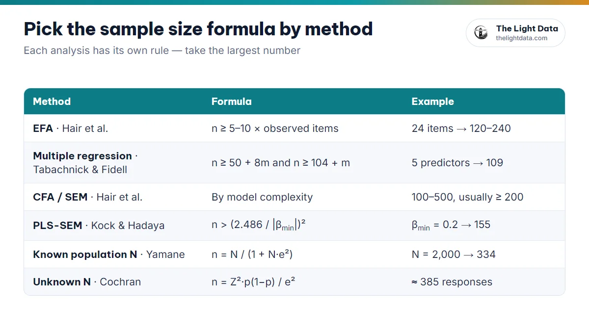
| Running EFA in SPSS | Hair et al.: n ≥ 5 × observed items |
| Multiple linear regression | Tabachnick & Fidell: n ≥ 50 + 8m |
| CFA or SEM in AMOS | By model complexity (Hair et al., 2019) |
| PLS-SEM in SmartPLS | Inverse square root (Kock & Hadaya, 2018) |
| Known population N (say, 2,000 students in a faculty) | Yamane / Slovin |
| Very large or unknown population | Cochran |
3Sample size for exploratory factor analysis
According to Hair, Black, Babin & Anderson (2019), factor analysis needs at least 50 observations, preferably 100 or more, with a minimum ratio of 5 observations per variable and preferably 10.
A model with 6 constructs of 4 items each has 24 items.
- 5:1 ratio → n ≥ 24 × 5 = 120
- 10:1 ratio → n ≥ 24 × 10 = 240
Count every item going into the EFA, including the dependent variable if you run them together. Demographic questions do not count.
4Sample size for multiple regression
Tabachnick & Fidell (2013) give two formulas, where m is the number of predictors:
- n ≥ 50 + 8m to test the overall model (R²).
- n ≥ 104 + m to test individual coefficients.
With 5 predictors: 50 + 8 × 5 = 90 and 104 + 5 = 109, so aim for at least 109 responses.
5Sample size for CFA and SEM in AMOS
CB-SEM (AMOS) is hungrier for data than regression because it estimates many parameters at once. Hair et al. (2019) tie the minimum to the complexity of the model:
| Model characteristics | Minimum sample |
|---|---|
| Up to 5 constructs, more than 3 items each, high communalities (≥ 0.6) | 100 |
| Up to 7 constructs, modest communalities (around 0.5) | 150 |
| Up to 7 constructs, low communalities (< 0.45) or constructs under 3 items | 300 |
| Many constructs with low communalities | 500 |
In practice, SEM studies usually aim for 200 responses or more so that fit indices behave.
6Sample size for PLS-SEM and SmartPLS
PLS-SEM copes better with smaller samples, but flexible does not mean anything goes.
The 10-times rule
Sample size ≥ 10 × the largest number of arrows pointing at any one construct (Barclay et al., 1995). It is easy to apply, but Hair et al. (2022) warn that it tends to underestimate the sample you need.
The inverse square root method (recommended)
From Kock & Hadaya (2018), recommended by Hair et al. (2022), at the 5% significance level:
nmin > (2.486 / |βmin|)², where βmin is the smallest path coefficient you expect to be significant, taken from earlier studies.
- βmin = 0.2 → (2.486 / 0.2)² = 154.5 → 155 responses
- βmin = 0.15 → (2.486 / 0.15)² = 274.7 → 275 responses
You can also run a power analysis in G*Power for multiple regression, using the largest number of predictors pointing at one construct, power of 0.80 and an effect size of f² = 0.15.
7Known population: the Yamane (Slovin) formula
When you can count the population (every student in a faculty, every employee of a company), use the Yamane (1967) formula, which some sources call the Slovin formula:
n = N / (1 + N × e²), where N is the population size and e the margin of error (usually 0.05).
For 2,000 students at e = 0.05: n = 2,000 / (1 + 2,000 × 0.0025) = 2,000 / 6 = 333.3 → 334 students.
8Unknown population: the Cochran formula
For a very large or uncountable population (say, “online shoppers in a city”), use the Cochran (1977) formula:
n = Z² × p × (1 − p) / e², with Z = 1.96 (95% confidence), p = 0.5 (the safest assumption) and e = 0.05.
n = 1.96² × 0.5 × 0.5 / 0.05² = 384.16 → 385 responses.
9Settling on a number and writing it up
Three steps:
- Calculate for each method you will use.
- Take the largest number as your minimum.
- Add a 10–20% reserve for responses you will discard during cleaning (incomplete, screened out, straight-lined).
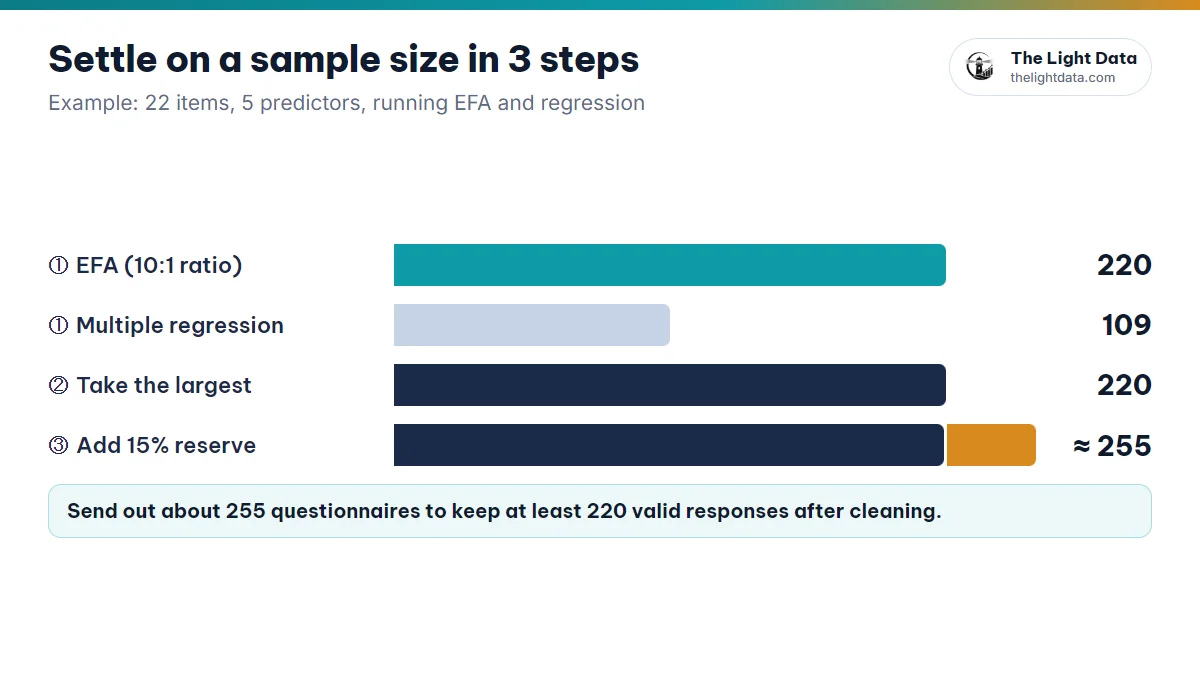
5 independent constructs plus 1 dependent, 22 items in total, running EFA and regression:
- EFA (10:1): 22 × 10 = 220
- Regression: max(50 + 8 × 5; 104 + 5) = 109
- → Minimum sample of 220; with a 15% reserve, send out about 255 questionnaires.
“According to Hair et al. (2019), the sample for exploratory factor analysis should have at least 5 observations per measured variable, and preferably 10. With 22 observed items, the minimum sample is 220. Tabachnick and Fidell (2013) indicate that multiple regression with 5 predictors requires at least 109 responses. To allow for invalid responses, 255 questionnaires were distributed.”
If you are short of responses, widen your channels or collect for longer. Fabricating or padding data is a breach of research integrity and can get a thesis invalidated.
Get ready faster with the right tools
- EFA: n ≥ 5–10 × observed items · Regression: n ≥ 50 + 8m and 104 + m.
- AMOS: by model complexity, usually ≥ 200 · SmartPLS: (2.486 / βmin)².
- Known population → Yamane; unknown → Cochran (about 385).
- Take the largest number, add 10–20% and state your reasoning in the thesis.