You open SPSS for the first time. It looks like a spreadsheet, but the menus are packed with jargon. What do you run first? Which table do you read? What Sig. value is good enough? This SPSS tutorial for beginners follows the 7-step path of a quantitative thesis, with thresholds, examples and the exact clicks at every step.
1What SPSS is and why theses use it
SPSS (Statistical Package for the Social Sciences) is IBM’s statistics software (IBM SPSS Statistics). You work through point-and-click menus with no coding, which is why it is so widely used in economics, management, education, psychology, sociology, health and marketing.
Strengths
- A friendly interface with clear menus
- Analyses from basic to advanced
- Easy tables and charts
- Widely accepted in theses and papers
Common uses
- Customer satisfaction and service quality surveys
- Consumer behavior and purchase intention
- Learning outcomes and teaching methods
- Comparing groups in health and social research
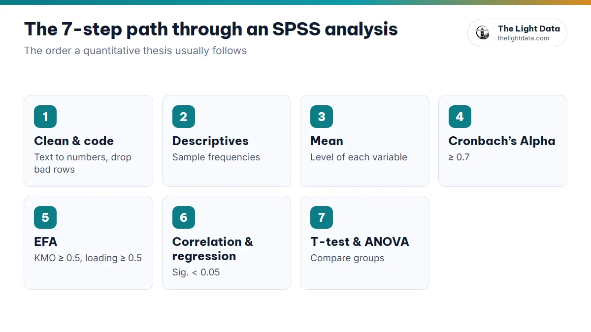
2The 7-step path through a thesis data analysis
A study using AMOS or SmartPLS still goes through steps ①–⑤ in SPSS (or moves to SmartPLS after step ②). See the AMOS tutorial and what SmartPLS is.
3Step 1: Clean and code your data
Your data needs preparing before any analysis, which involves five jobs:
- Check the data: sample size, missing values, entry errors, duplicates
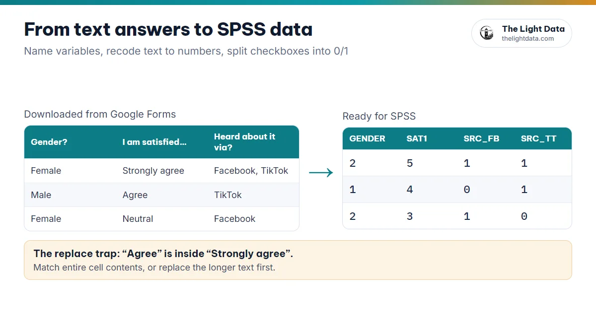
- Code variables: turn answers into numbers (Male = 1, Female = 2; Likert 1–5)
- Declare variables in Variable View: Name, Label, Values, Missing, Measure
- Check outliers: boxplot, Explore, z-scores
- Save as .sav
Coding a Likert scale in the wrong direction or forgetting to reverse-code an item breaks every analysis that follows, and SPSS gives no warning.
4Step 2: Descriptive statistics
Summarize your sample: gender, age, income and so on. This is usually the first table of your results chapter.
A survey of 200 students:
| Gender | Count | Percent |
|---|---|---|
| Male | 90 | 45 |
| Female | 110 | 55 |
- Categorical variables: Analyze→Descriptive Statistics→Frequencies
- Quantitative variables: Analyze→Descriptive Statistics→Descriptives → Options: Mean, SD, Min, Max
5Step 3: Means of Likert scales
Show the average rating for each variable or construct, along with its standard deviation. For a 5-point scale, one common way to interpret it:
- Mean < 2.5: Low
- 2.5 to < 3.5: Moderate
- Mean ≥ 3.5: High
“I am satisfied with the quality of teaching”: Mean = 4.12, SD = 0.68. Respondents tend to agree.
6Step 4: Cronbach’s alpha reliability test
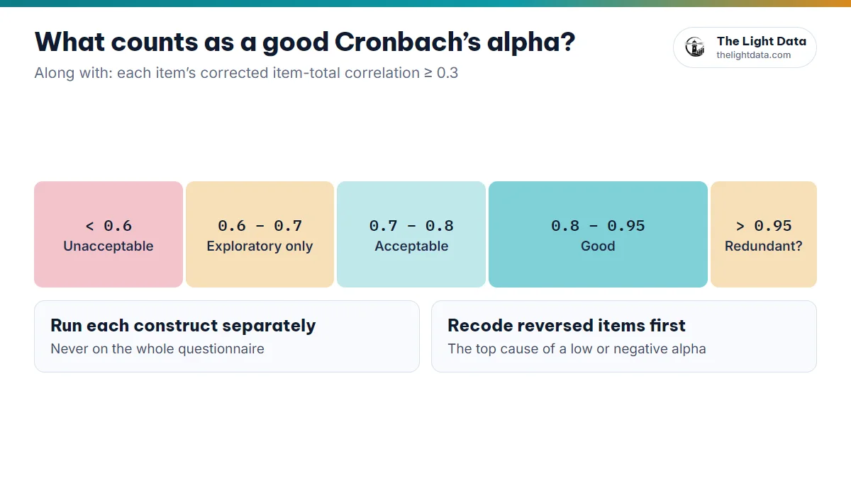
Check that items in the same construct measure consistently. The standard: alpha ≥ 0.7 (≥ 0.6 for exploratory research) and item-total correlation ≥ 0.3.
- Analyze→Scale→Reliability Analysis
- Statistics: Item, Scale, Scale if item deleted. Run each construct separately.
7Step 5: Exploratory factor analysis
Check the convergent and discriminant validity of your scales once they pass Cronbach’s alpha.
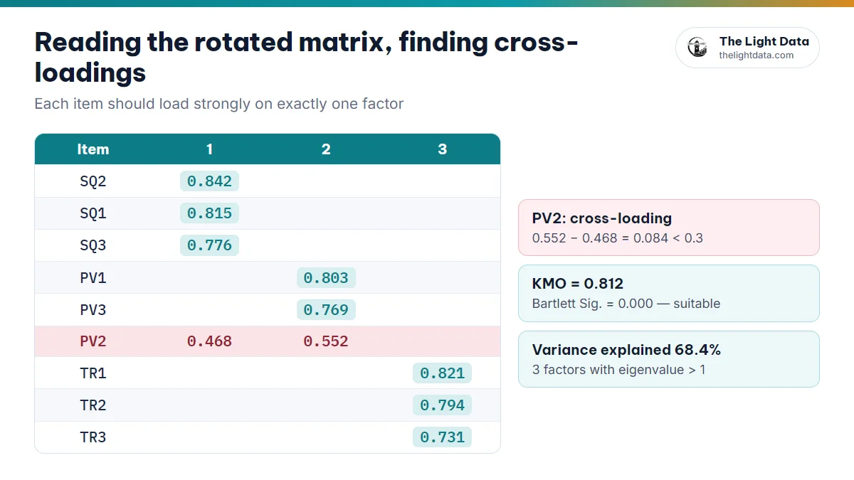
- KMO ≥ 0.5 · Bartlett Sig. < 0.05
- Eigenvalue > 1 · Variance explained ≥ 50%
- Loading ≥ 0.5, with each item on exactly one factor
- Analyze→Dimension Reduction→Factor
- Descriptives: KMO and Bartlett · Extraction: Principal components, Eigenvalue > 1 · Rotation: Varimax · Options: Sorted by size, Suppress 0.3
8Step 6: Pearson correlation and multiple regression
Pearson correlation
Shows the strength and direction of linear relationships between variables (r from −1 to 1). Sig. < 0.05 means the correlation is significant. Predictors should correlate significantly with the dependent variable; very high correlations among predictors (above about 0.8) suggest multicollinearity.
- Analyze→Correlate→Bivariate → Pearson · Two-tailed
Multiple linear regression
Measures how much each predictor affects the dependent variable and tests your hypotheses.
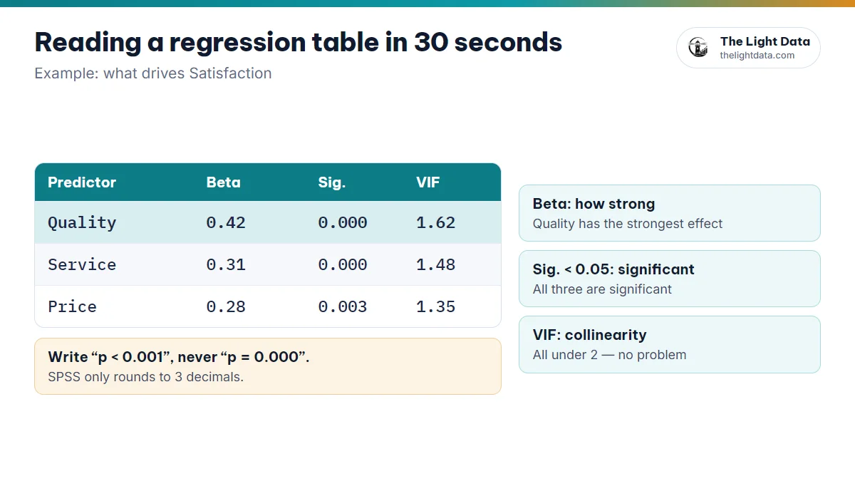
| Predictor | Standardized Beta | Sig. | VIF |
|---|---|---|---|
| Quality | 0.42 | .000 | 1.62 |
| Service | 0.31 | .000 | 1.48 |
| Price | 0.28 | .003 | 1.35 |
All three have a significant positive effect (Sig. < 0.05); Quality is the strongest (largest Beta); VIF under 2 means no multicollinearity.
- Normal residuals: histogram, normal P-P plot.
- Constant residual variance: a scatterplot of standardized residuals against standardized predicted values.
- No multicollinearity: low VIF (usually under 10; stricter guidance says under 5 or 3).
- Independent residuals: Durbin–Watson around 1.5–2.5.
- Analyze→Regression→Linear
- Statistics: Estimates · Model fit · Collinearity diagnostics · Durbin-Watson
- Plots: ZRESID (Y) against ZPRED (X) · Histogram · Normal probability plot
9Step 7: Comparing groups with t-tests and ANOVA
Test whether groups (gender, age, income) differ on the mean of a variable.
Independent samples t-test: 2 groups
Read Levene’s test first: Levene Sig. ≥ 0.05 means read the Equal variances assumed row, and < 0.05 means read not assumed. Then Sig. (2-tailed) < 0.05 means the groups differ.
- Analyze→Compare Means→Independent-Samples T Test
- Test Variable: the quantitative variable · Grouping Variable: the group → Define Groups: 1 and 2
One-way ANOVA: 3 or more groups
Levene Sig. ≥ 0.05: read the ANOVA table and follow up with Tukey or Bonferroni. Levene Sig. < 0.05: read the Welch test (Robust Tests) and use Games-Howell post hoc.
- Analyze→Compare Means→One-Way ANOVA
- Options: Descriptive · Homogeneity of variance test · Welch
- Post Hoc: Tukey (equal variances) · Games-Howell (unequal)
105 mistakes SPSS beginners make
| Mistake | What to do instead |
|---|---|
| Reporting “p = .000” | Report “p < .001”, since SPSS only rounds to 3 decimals |
| Running Cronbach’s alpha on the whole questionnaire | Run it for each construct |
| Automatic Recode on Likert items | Recode into Different Variables with an explicit mapping |
| Skipping Levene’s test in t-tests and ANOVA | Read Levene first to pick the right row or test |
| Putting single items into regression instead of construct scores | Create a score: Transform → Compute Variable → MEAN(SQ1, SQ2, SQ3) |
Learn faster with simulated data
Want to see the SPSS tables for your own model (alpha, rotated matrix, correlation, regression) before you have data? Draw it on The Light Data’s model canvas and read the results on simulated data. It is for learning only and never replaces real data.
- The path: clean and code → descriptives → means → alpha → EFA → correlation and regression → t-test and ANOVA.
- Clear thresholds at every step: alpha ≥ 0.7 · KMO ≥ 0.5 · loading ≥ 0.5 · Sig. < 0.05 · low VIF.
- Check the regression assumptions and Levene’s test before you conclude.